Reading-notes
Trees
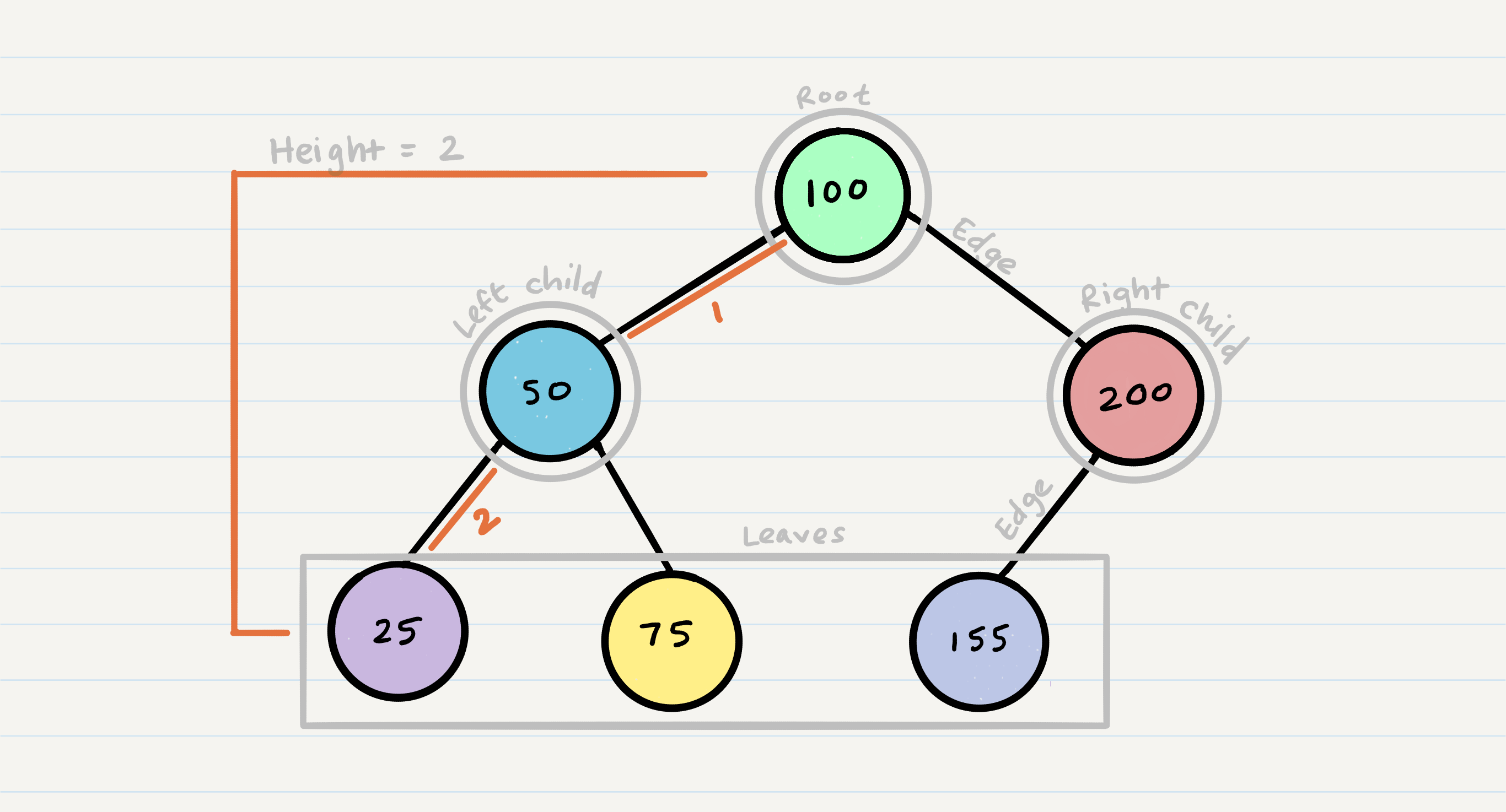
Common Terminology
-
Node - A Tree node is a component which may contain it’s own values, and references to other nodes
-
Root - The root is the node at the beginning of the tree
-
K - A number that specifies the maximum number of children any node may have in a k-ary tree. In a binary tree, k = 2.
-
Left - A reference to one child node, in a binary tree
-
Right - A reference to the other child node, in a binary tree
-
Edge - The edge in a tree is the link between a parent and child node
-
Leaf - A leaf is a node that does not have any children
-
Height - The height of a tree is the number of edges from the root to the furthest leaf
Traversing a tree
The most common way to traverse through a tree is to use recursion
Traversing a tree allows us to search for a node, print out the contents of a tree, and much more! There are two categories of traversals.
** The biggest difference between each of the traversals is when you are looking at the root node.**
## Depth First ( prioritize going through the depth (height) of the tree first.)
## ** methods for depth first traversal:**
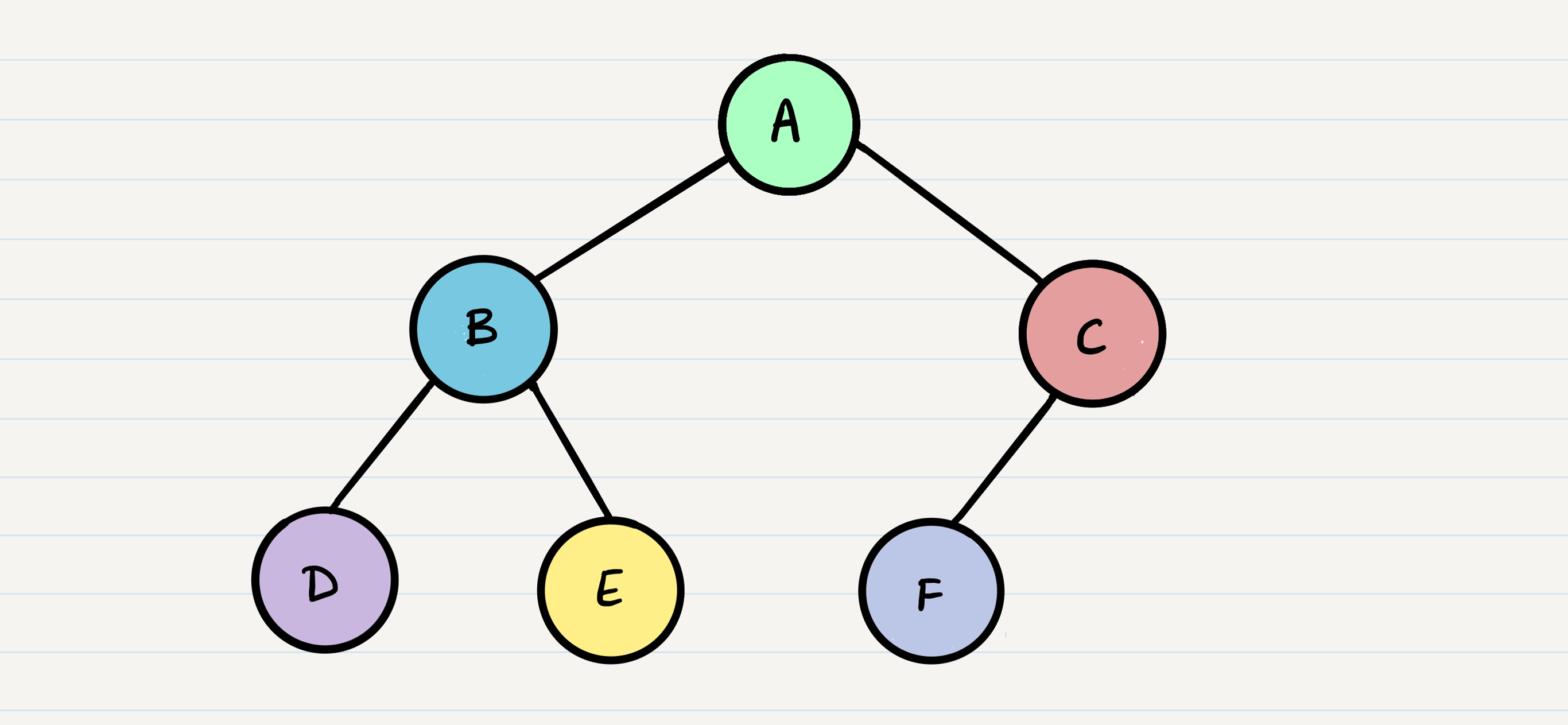
Pre-order: root >> left >> right
Pre-order
ALGORITHM preOrder(root)
// INPUT <-- root node
// OUTPUT <-- pre-order output of tree node's values

    OUTPUT <-- root.value

    if root.left is not Null
        preOrder(root.left)

    if root.right is not NULL
        preOrder(root.right)
In-order: left >> root >> right
In-order
ALGORITHM inOrder(root)
// INPUT <-- root node
// OUTPUT <-- in-order output of tree node's values

    if root.left is not NULL
        inOrder(root.left)

    OUTPUT <-- root.value

    if root.right is not NULL
        inOrder(root.right)
Post-order: left >> right >> root
Post-order
ALGORITHM postOrder(root)
// INPUT <-- root node
// OUTPUT <-- post-order output of tree node's values

    if root.left is not NULL
        postOrder(root.left)

    if root.right is not NULL
        postOrder(root.right)

    OUTPUT <-- root.value
Pre-order
Pre-order means that the root has to be looked at first
Breadth First
iterates through the tree by going through each level of the tree node-by-node.
uses a queue (instead of the call stack via recursion) to traverse the width/breadth of the tree. Let’s break down the process.
**output is [A, B, C, D, E, F]
Pseudocode
``` ALGORITHM breadthFirst(root) // INPUT <-- root node // OUTPUT <-- front node of queue to console
Queue breadth <– new Queue() breadth.enqueue(root)
while breadth.peek() node front = breadth.dequeue() OUTPUT <– front.value
if front.left is not NULL
  breadth.enqueue(front.left)

if front.right is not NULL
  breadth.enqueue(front.right)
  ```
Binary Tree Vs K-ary Trees
Binary Trees restrict the number of children to two (hence our left and right children).
If Nodes are able have more than 2 child nodes, we call the tree that contains them a K-ary Tree.
Traversing a K-ary
equires a similar approach to the breadth first traversal. but we are now moving down a list of children of length k, instead of checking for the presence of a left and a right child.
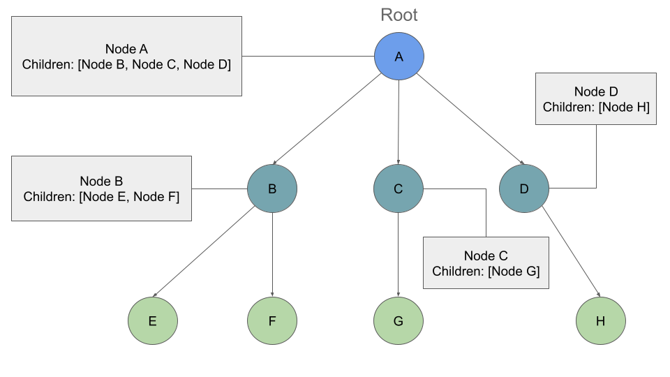
Output: A, B, C, D, E, F, G, H
Pseudocode
’’’ ALGORITHM breadthFirst(root) // INPUT <– root node // OUTPUT <– front node of queue to console
Queue breadth <– new Queue() breadth.enqueue(root)
while breadth.peek() node front = breadth.dequeue() OUTPUT <– front.value
for child in front.children
    breadth.enqueue(child) '''
Adding a node
Because there are no structural rules for where nodes are “supposed to go” in a binary tree, it really doesn’t matter where a new node gets placed.
In the event you would like to have a node placed in a specific location, you need to reference both the new node to create, and the parent node upon which the child is attached to.
A “perfect” binary tree is one where every non-leaf node has exactly two children
Big O
The Big O time complexity for inserting a new node is O(n). Searching for a specific node will also be O(n)
Binary Search Trees
A Binary Search Tree (BST) is a type of tree that does have some structure attached to it
nodes are organized in a manner where all values that are smaller than the root are placed to the left, and all values that are larger than the root are placed to the right.
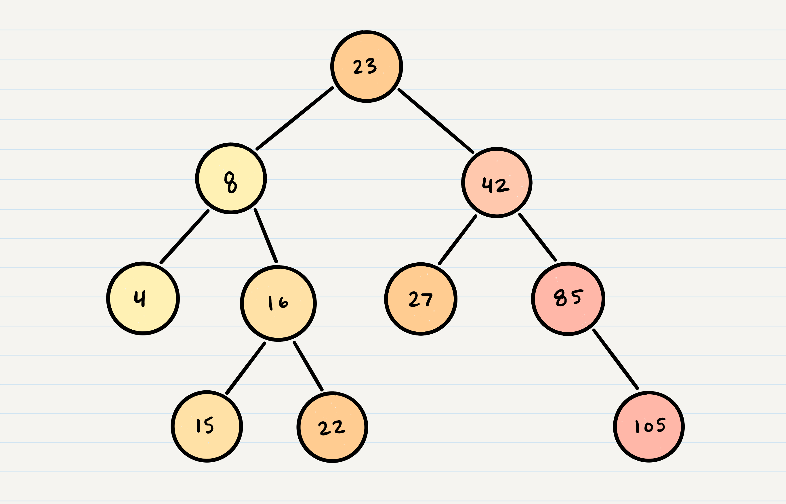
Searching a BST
Searching a BST can be done quickly, because all you do is compare the node you are searching for against the root of the tree or sub-tree.
ex: If the value is smaller, you only traverse the left side. If the value is larger, you only traverse the right side.
the Big O time complexity of a Binary Search Tree’s insertion and search operations is O(h), or O(height)